Definition by sound example
The goal of this section is to orient everyone towards the general concepts involved in the estimation of tempo, beat, and downbeats from musical audio signals.
While this could be acheived through an extensive literature review supported by the diverse multi-disciplinary perspectives including music theory, psychology, and cognitive neuroscience, we instead try to provide a quick and intuitive means to grasp the relevant concepts via a set of three annotated sound examples. Where appropriate we draw upon the relevant different multi-disciplinary perspectives, as a means to demonstrate the interestingness of the tasks and the potential challenges when addressing them in a computational manner.
A straightforward example
Let’s start with a relatively easy example which should help clarify what the intuitive target is for a system that can estimate the metrical structure of a piece of music. For this example we can plot the waveform and listen to the audio excerpt.
Task
Why not go ahead and try to tap the beat yourself? You can also try to count along as well.
# Do import and setup
import warnings
warnings.simplefilter('ignore')
import matplotlib.pyplot as plt
%matplotlib inline
import numpy as np
from pprint import pprint
import librosa
import librosa.display
import IPython.display as ipd
SR = 44100
FIGSIZE = (14,3)
x1, sr = librosa.load('../assets/ch2_basics/audio/easy_example.flac', sr = SR)
plt.figure(figsize=FIGSIZE)
librosa.display.waveplot(x1, sr=SR, alpha=0.6); # this semi-colon surpresses the matplotlib stdout <matplotlib.zzz.zzz at 0x etc.>
plt.title('Easy Example: audio waveform', fontsize=15)
plt.yticks(fontsize=12)
plt.xticks(fontsize=12)
plt.xlabel('Time', fontsize=13)
plt.xlim(0, len(x1)/sr);
ipd.Audio(x1, rate=SR)
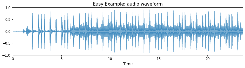
Wait! What is that amazing song?
“Shampoo” from the album “Shampoo” by Yuko Tomita
At the time of writing, you can listen to the full version on YouTube

What we’re trying to work towards in this tutorial is to design and execute a deep learning based system that can “listen” to pieces of music like this and then not only tap along to mark the beat, but also count in time to music.
Essentially this means that it can discover a quasi-periodic sequence of time-points which convey the most comfortable rate at which to tap along to the piece, and their metrical organisation, i.e., the grouping of beats into bars. The tempo can then be understood as the number of beats per minute, which is to say an indication as to whether the music is fast, meaning it has many beats per minute and hence a high tempo, or alternatively if the piece is slow and has a lower number of beats per minute.
Now let’s look at the waveform again with the beats and downbeats drawn on top, and also listen to them rendered as short pulses. The higher pitched pulses correspond to the downbeat or the “1” of every bar, and the lower pitched pulses correspond to the remaining beats in each bar.
beats1 = np.loadtxt('../assets/ch2_basics/audio/easy_example.beats')
downbeats1 = beats1[beats1[:, 1] == 1][:, 0]
beats1 = beats1[:,0]
y_beats1 = librosa.clicks(times=beats1, sr=SR, click_freq=1000.0, click_duration=0.1, click=None, length=len(x1))
y_downbeats1 = librosa.clicks(times=downbeats1, sr=SR, click_freq=1500.0, click_duration=0.15, click=None, length=len(x1))
plt.figure(figsize=FIGSIZE)
librosa.display.waveshow(x1, sr=SR, alpha=0.6)
plt.vlines(beats1, 1.1*x1.min(), 1.1*x1.max(), label='Beats', color='r', linestyle=':', linewidth=2)
plt.vlines(downbeats1, 1.1*x1.min(), 1.1*x1.max(), label='Downbeats', color='black', linestyle='--', linewidth=2)
plt.legend(fontsize=12);
plt.title('Easy example: audio waveform with beats and downbeats', fontsize=15)
plt.yticks(fontsize=12)
plt.xticks(fontsize=12)
plt.xlabel('Time', fontsize=13)
plt.xlim(0, len(x1)/sr);
ipd.Audio(0.6*x1+0.25*y_beats1+0.25*y_downbeats1, rate=SR)
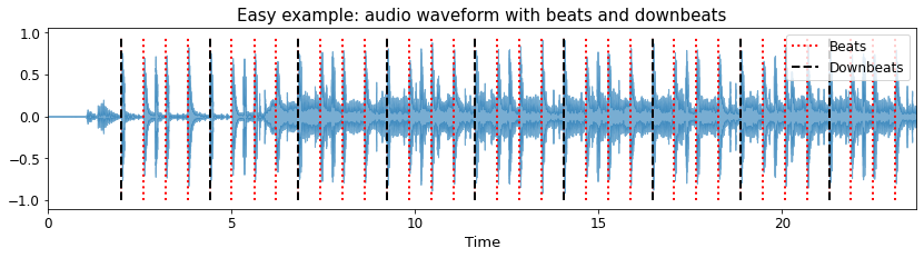
Our intent is for this example to be relatively unambiguous in terms of the placement of the beats, and thus the “preferred” metrical level at which to tap. The beats are evenly spaced at a tempo of 100 beats per minute (bpm) and with a constant 4/4 metre. The clear presence of drums with a repeating pattern of a kick drum events on the ‘1’ and ‘3’ and snare drum events on the ‘2’ and ‘4’ makes for a pretty straightforward excerpt both for human tappers and likewise for a computational system. In addition there are chord changes which also assist in understanding the harmonic rhythm of the piece.
Having said that, outside of trivial cases (e.g., an isolated metronome), there is almost never likely to be complete agreement among tappers of the metrical level. Some people may prefer to tap at a slower rate (e.g., at half the tempo), while others may tap twice as fast. Alternatively some tappers might tap the so-called “off-beat” corresponding to the same tempo, but tapping in the mid-way point between each beat, i.e., shifted by one 1/8th note.
An expressive example
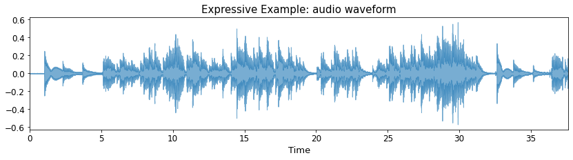
Having looked at an easy example, let’s transition to a more complicated case. As before, we’ll begin by looking at the waveform and listening the audio excerpt. The piece in question is the Heitor Villa-Lobos composition Choros №1 as performed by Kyuhee Park
Once again you can have a go tapping and counting along with the piece.
Note
Since the code examples are more or less identical for the remaining sound examples they’re hidden by default, but clicking the plus symbol on the right hand side next to where it says “Click to show” will reveal them.
x2, sr = librosa.load('../assets/ch2_basics/audio/expressive_example.flac', sr = SR)
plt.figure(figsize=FIGSIZE)
plt.title('Expressive Example: audio waveform', fontsize=15)
plt.yticks(fontsize=12)
plt.xticks(fontsize=12)
plt.xlabel('Time', fontsize=13)
plt.xlim(0, len(x2)/sr);
librosa.display.waveshow(x2, sr=SR, alpha=0.6);
ipd.Audio(x2, rate=SR)
What’s different?
There are no drums, just a guitarist playing alone
So no need to synchronise with anyone else
In this sense there is no need for a “shared sense” of the beat
The tempo is not constant, and there are some big pauses to deal with!
This makes it harder to predict the next beat - especially on the first listen
Computationally, this also means that the tempo must be tracked through time as opposed to a single, global estimate
What’s the same?
While the musical content is completely different, the goal is unchanged:
Try to tap your foot in time with the beat and count the metrical positions
Thus, at a high level, the formulation of problem from a computational perspective is the same:
audio-in, beats+dowbeats-out
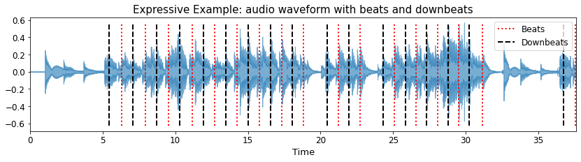
Let’s take a listen again, but this time with the beat and downbeat markers rendered as short pulses:
beats2 = np.loadtxt('../assets/ch2_basics/audio/expressive_example.beats')
downbeats2 = beats2[beats2[:, 1] == 1][:, 0]
beats2 = beats2[:,0]
y_beats2 = librosa.clicks(times=beats2, sr=SR, click_freq=1000.0, click_duration=0.1, click=None, length=len(x2))
y_downbeats2 = librosa.clicks(times=downbeats2, sr=SR, click_freq=1500.0, click_duration=0.15, click=None, length=len(x2))
plt.figure(figsize=FIGSIZE)
librosa.display.waveshow(x2, sr=SR, alpha=0.6)
plt.vlines(beats2, 1.1*x2.min(), 1.1*x2.max(), label='Beats', color='r', linestyle=':', linewidth=2)
plt.vlines(downbeats2, 1.1*x2.min(), 1.1*x2.max(), label='Downbeats', color='black', linestyle='--', linewidth=2)
plt.legend(fontsize=12);
plt.title('Expressive Example: audio waveform with beats and downbeats', fontsize=15)
plt.yticks(fontsize=12)
plt.xticks(fontsize=12)
plt.xlabel('Time', fontsize=13)
plt.legend(fontsize=12);
plt.xlim(0, len(x2)/sr);
ipd.Audio(0.6*x2+0.25*y_beats2+0.25*y_downbeats2, rate=SR)
Do you agree with the annotations?
Did you prefer to tap at a faster or slower rate?
Maybe you kept this tempo, but counted the beats in groups of four rather than two?
Maybe you felt the timing of the taps was a little off? Especially on the first beat!
Wait, why are there no beats in the first 5 seconds of the piece?
In order to try to address these points we need to consider how this annotation was made. We’ll see more about “how to annotate” in the next section, but for now we can make some headway in addressing these points by looking at a score representation for the very beginning of the piece.
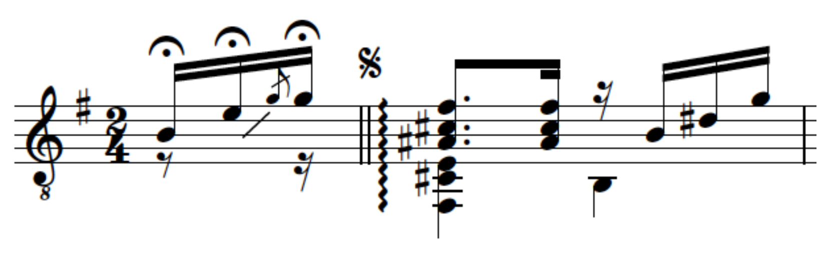
Without wishing to get too technical in musical terms, the score shows that the first three notes of the piece, corresponding to its main motif, form an anacrusis - meaning a “lead-in” to the first complete bar, and are notated to be played in a very expressive manner at the discretion of the performer. While these three notes take up almost the first 5 seconds of the piece, from a music notation perspective they are all 1/16th notes, and thus all fall within a single notated beat (i.e., one 1/4 note). On this basis, if we are to rely on the score, then none of the notes should be tapped at the start, nor when the motif repeats around the 30s mark.
The score also tells us the time-signature of the piece is 2/4 and thus we should count the beats in groups of 2 rather than 4. This also lets us know which notes correspond to the beat-level and thus the rate at which we should tap (again, if we want to stick to the score).
Finally, concerning the beginning of the first complete bar, i.e., the point at which the first overlaid pulse can be heard, this corresponds to an arpeggiated chord, where the plucking of the strings is not simultaneous, but drawn out so the individual notes of the chord can be heard. Again, notationally these notes correspond to a single beat, but this elongation of the chord makes it difficult to precisely identify a single time instant to mark as the beat.
In summary, if we rely on the score then this can help guide how the annotation should be performed. On the other hand, tapping purely based on listener perception, especially without prior familiarity with the peice, could lead to different annotations.
A nonwestern example
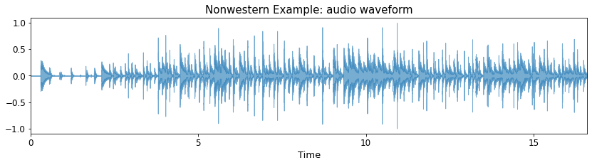
In our final example let’s move away from “western” music and consider an excerpt of Uruguayan Candombe (taken from the Candombe Recordings Dataset. As before, please also have a go tapping and counting along!
x3, sr = librosa.load('../assets/ch2_basics/audio/nonwestern_example.flac', sr = SR)
plt.figure(figsize=FIGSIZE)
librosa.display.waveshow(x3, sr=SR, alpha=0.6);
plt.title('Nonwestern Example: audio waveform', fontsize=15)
plt.yticks(fontsize=12)
plt.xticks(fontsize=12)
plt.xlim(0, len(x3)/sr);
plt.xlabel('Time', fontsize=13)
ipd.Audio(x3, rate=SR)
Let’s now listen to the expert annotations.
beats3 = np.loadtxt('../assets/ch2_basics/audio/nonwestern_example.beats')
downbeats3 = beats3[beats3[:, 1] == 1][:, 0]
beats3 = beats3[:,0]
y_beats3 = librosa.clicks(times=beats3, sr=SR, click_freq=1000.0, click_duration=0.1, click=None, length=len(x3))
y_downbeats3 = librosa.clicks(times=downbeats3, sr=SR, click_freq=1500.0, click_duration=0.15, click=None, length=len(x3))
plt.figure(figsize=FIGSIZE)
librosa.display.waveshow(x3, sr=SR, alpha=0.6)
plt.vlines(beats3, -1, 1, label='Beats', color='r', linestyle=':', linewidth=2)
plt.vlines(downbeats3, -1, 1, label='Downbeats', color='black', linestyle='--', linewidth=2)
plt.title('Nonwestern Example: audio waveform with beats and downbeats', fontsize=15)
plt.yticks(fontsize=12)
plt.xticks(fontsize=12)
plt.xlabel('Time', fontsize=13)
plt.legend(fontsize=12);
plt.xlim(0, len(x3)/sr);
ipd.Audio(0.6*x3+0.25*y_beats3+0.25*y_downbeats3, rate=SR)
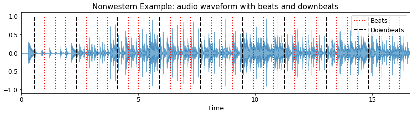
The specific challenge here lies not only in the rhythmic density of the performance, but in understanding the metrical organisation. For those familiar with Candombe this is a straightforward excerise and as such it can be tapped and counted in an unambiguous way, but to the untrained ear (or algorithm!) it can be much more challenging to understanding how to tap along.
As we proceed through the remainder of this part of the tutorial we’ll revisit these examples again when we look at a baseline approach and also explore the means by which algorithms can be evaluated.
Summary
In this section we’ve looked at three different sound examples as a means to intuitively understand the nature, interestingness, and challenges of the tasks of tempo, beat, and downbeat estimation.
While we’ve touched upon it here, we’ll now move on to considering the process of annotation in more detail.