Post-processing¶

Ideally the output likelihood of a DNN would be a robust estimation of the positions of beats and downbeats, but in practice likelihoods are noisy, and just post-processing them using peak-picking or a simple threshold would not be enough to obtain a musically consistent sequence. To obtain a reasonable estimation of beat and downbeat positions, most methods use a Probabilistic Graphical Models (PGMs) as post-processing of a likelihood from a DNN, as they allow to easily and intuitively encode musical-consistency constrains at inference time.

Fig. 15 Post-processing the likelihood from a DNN.¶

Probabilistic graphical models¶

PGMs are a set of probabilistic models that express conditional dependencies between random variables as a graph. This graph can be directed, carrying a causal interpretation, or undirected, where there are no causal influences represented (see Figure below). In directed graphs, the concept of parent nodes refers to nodes that precede topologically the others.

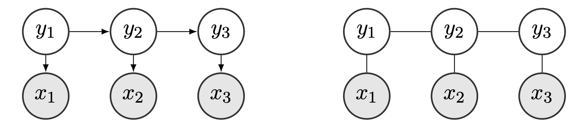
Example of a directed graph (left) and an undirected (right).

Fig. 16 Example of directed graph (left) and undirected graph (right).¶

In the context of classification problems, the objective is to assign classes to observed entities. Two approaches commonly used in the context of sequential data classification are generative and discriminative models. Generative models are concerned with modelling the joint probability $P(\textbf{x},\textbf{y})$ given the input and output sequences $\textbf{x}$ and $\textbf{y}$. They are generative in the sense that they describe how the output probabilistically generates the input, and the main advantage of this approach is that it is possible to generate samples from it (i.e. to generate synthetic data that can be useful in many applications). The main disadvantage of generative models is that to use them in classification tasks, where the ultimate goal is to obtain the sequence that maximizes $P(\textbf{y}|\textbf{x})$ (the most probable output given the input), one needs to model the likelihood $P(\textbf{x}|\textbf{y})$. Modelling $P(\textbf{x}|\textbf{y})$ can be very difficult when data involves very complex interrelations, but also simplifying them or ignoring such dependencies can impact the performance of the model [SM12]. In applications where generating data is not intended, it is more efficient to use discriminative models, which directly model the conditional probability between inputs and outputs $P(\textbf{y}|\textbf{x})$. The main advantage of these models is that relations that only involve $\textbf{x}$ play no role in the modelling, usually leading to compact models with simpler structure than generative models.

Note

In the context of beat and downbeat tracking both types of models –generative and discriminative– have been used leading to similar results.

PGMs have been explored across different MIR tasks given their capacity to deal with structure in a flexible manner. In the following we introduce the main models exploited in the literature and their motivation, instantiating relevant works.

Hidden Markov Models¶

Hidden Markov models (HMMs) [Rab89] are the most common graphical models used for music processing [PT16], in particular in rhythm analysis [DBDR16, SHCS15] and widely used in the context of speech analysis and sequential problems in general. HMMs are generative models, so they compute the joint probability $P(\textbf{x},\textbf{y})$ between a sequence of $T$ hidden states $\textbf{y}$ and a sequence of observations $\textbf{x}$. A HMM makes two important independence assumptions:

each observation $x_t$ depends only on the current state $y_t$,
each state $y_t$ depends only on its immediate predecessor $y_{t-1}$, which is called the Markovian assumption.

The joint probability of the state sequence $\textbf{y}$ and the observation sequence $\textbf{x}$ in an HMM factorizes as a product of conditional probabilities, given by the parent node in the direct graph as:

\[ P(\mathbf{y},\mathbf{x}) = P(y_1)\prod _{t=2} ^T P(y_t|y_{t-1})P(x_t|y_t), \]

where $P(y_t|y_{t-1})$ is the transition probability, $P(x_t|y_t)$ is the observation probability, and $P(y_1)$ is the distribution over initial states.

Rhythm analysis problems such as beat or downbeat tracking can be seen as sequence labelling problems, so that given a sequence of observations, the objective is to assign a pre-defined class to each one of these events. In the context of HMMs, this translates to finding the maximum likelihood sequence $\textbf{x}^*$ that maximizes $P(\textbf{x}|\textbf{y})$, that is:

\[ \textbf{x}^* = \mbox{arg}\: \mbox{max}_{x}P(\textbf{x}|\textbf{y}) \]

The most common algorithm used to solve this is the Viterbi algorithm [Rab89].

Dynamic Bayesian Networks¶

Dynamic Bayesian Networks (DBNs) [MR02] are a generalization of HMMs. DBNs are Bayesian Networks that relate variables to each other over adjacent time steps. Like HMMs, they represent a set of random variables and their conditional dependencies with a directed acyclic graph, but they are more general than HMMs since they allow one to model multiple hidden states. Given the hidden and observed sequences of variables $\textbf{y}$ and $\textbf{x}$ of length $T$, the joint probability of the hidden and observed variables factorizes as:

\[ P(\textbf{y},\textbf{x})=P(\textbf{y}_1)\prod ^T _{t=2}P(\textbf{y}_t | \textbf{y}_{t-1})P(\textbf{x}_t | \textbf{y}_t), \]

with $P(\textbf{y}_t | \textbf{y}_{t-1})$, $P(\textbf{x}_t | \textbf{y}_t)$ and $P(\textbf{y}_1)$ the transition probability, observation probability and initial states distribution as an HMM, but over a set of hidden variables. The initial state distribution is usually set to a uniform initialization in practice.

DBNs provide an effective framework to represent hierarchical relations in sequential data, as it is the case of musical rhythm. Probably the most successful example is the bar pointer model (BPM) [WCG06], which has been proposed by Whiteley et al. for the task of meter analysis and has been further extended in recent years [HKS14, KBockDW16, KBockW13, SHCS15, SHCS16]. A short overview of it and one of its relevant variants is presented in the following. Given that there are multiple versions of this model, we chose the variant presented in [SHCS15] for this explanation.

The Bar Pointer Model¶

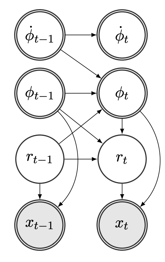
Fig. 17 Bar Pointer Model as it appears in [SHCS15]. Double circles denote continuous variables, and simple circles denote discrete variables. The gray nodes are observed, and the white nodes represent hidden variables.¶

The BPM describes the dynamics of a hypothetical pointer that indicates the position within a bar, and progresses at the speed of the tempo of the piece, until the end of the bar where it resets its value to track the next bar. A key assumption in this model is that there is an underlying bar-length rhythmic pattern that depends on the style of the music piece, which is used to track the position of the pointer.

The effectiveness of this model relies on its flexibility, since it accounts for different metrical structures, tempos and rhythmic patterns, allowing its application in different music genres ranging from Indian music to Ballroom dances [HKS14, SHCS16].

Hidden states¶

The hidden state $\textbf{y}_t$ represents the position of the hypothetical pointer at each time frame $t$, and is given by $\textbf{y}_t=[\phi_t\:\: \dot{\phi}_t \:\: r_t]$, where each variable describes the position inside the bar, the instantaneous tempo, and the rhythmic pattern respectively.

$r_t \in {r_1 \ldots r_R}$ is a rhythmic pattern indicator that can be used to differentiate between $R$ different rhythmic patterns, which can be known a priori or learned.
The variable $\phi _t \in [0,M_{r_t})$ is the current position in a bar, and $M_{r_t}$ is the length of a bar related to the considered rhythmic patterns. Different rhythmic patterns associated to different time signatures or meter cycles will have different number of discrete positions. Common practice is to fix the length of one time signature or meter cycle and scale the rest accordingly.
$\dot{\phi}_t \in [\dot{\phi}_{min},\:\dot{\phi}_{max}]$ is the instantaneous tempo (denoting the rate at which the bar pointer traverses a bar). $\dot{\phi}_t$ is given by the number of bar positions per frame. The tempo limits are assumed to depend on the rhythmic pattern state.

Transition Model¶

Due to the conditional independence relations shown in Figure \ref{fig:bpm}, the transition model factorizes as: $$ P(\textbf{y}_t | \textbf{y}_{t-1})=P(\phi_t | \phi_{t-1},\dot{\phi}_{t-1},r_{t-1})\times P(\dot{\phi}_t | \dot{\phi}_{t-1})\times P(r_t | r_{t-1}, \phi_{t-1}, \phi_t), $$ where the three factors are defined as:

$P(\phi _t | \phi _{t-1},\dot{\phi}_{t-1},r_{t-1})=1_\phi$, where $1_\phi$ is an indicator function that equals one if $\phi _t=(\phi _{t-1}+\dot{\phi}_{t-1})\: \mbox{mod} \: M_{r_t}$ and $0$ otherwise.
The tempo transition from one frame to the next is assumed to follow a normal distribution and is given by: $P(\dot{\phi}_t |\dot{\phi}_{t-1})\propto \mathcal{N}(\dot{\phi} _{t-1}, \sigma ^2 _{\dot{\phi}})\times 1_{\dot{\phi}}$, where $\sigma _{\dot{\phi}}$ is the standard deviation of the tempo transition model and $1_{\dot{\phi}}$ is an indicator function that equals one if $\dot{\phi_t} \in [\dot{\phi_{min}}, \dot{\phi_{max}}]$, and $0$ otherwise.
$P(r_t | r_{t-1},\phi_{t-1}, \phi_t)= \left\{ \begin{array}{@{} l l @{}} \mathcal{A}(r_t, r_{t-1}) & \hspace{-0.2cm}\mbox{if}\: \phi_t < \phi_{t-1},\\ 1_r & \hspace{-0.15cm} \mbox{otherwise}, \end{array}\right .$, where $\mathcal{A}(i,j)$ is the transition probability from $r_i$ to $r_j$, and $1_r$ is an indicator function that equals one when $r_t=r_{t-1}$ and $0$ otherwise.

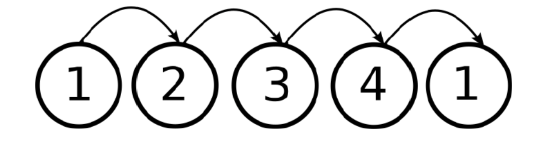
Fig. 18 Transitions between states are cyclic in the BPM.¶

Observation model¶

The observation model $P(\textbf{x}_t|\textbf{y}_t)=P(\textbf{x}_t| \phi_t, r_t)$ proposed in [SHCS15] is given by learned features using GMMs with two components. Among the variations of the BPM, other observation models have been proposed using RNNs [BockKW16, KBockW11].

Inference¶

The inference of a model with continuous variables is usually done approximately, where sequential Monte Carlo (SMC) algorithms have been explored in the context of rhythm analysis [KHCW15, SHCS15]. It is also common to discretize the variables $\dot{\phi}_t$ and $\phi_t$, and then perform the inference using Viterbi.

Conditional Random Fields¶

Conditional Random Fields (CRFs) are a particular case of undirected PGMs. Unlike generative models such as HMMs, which model the joint probability of the input and output $P(\textbf{x},\textbf{y})$, CRFs model the conditional probability of the output given the input $P(\textbf{y}|\textbf{x})$. CRFs can be defined in any undirected graph, making them suitable to diverse problems where structured prediction is needed across various fields, including text processing [Set05, SP03], computer vision [HZCPerpinan04, KH04] and combined applications of NLP and computer vision [ZZH+17].

Beat and downbeat tracking are sequential problems, i.e. the variables involved have a strong dependency over time. Equations below present a generic CRF model for sequential problems, where $\Psi _k$ are called potentials, which act in a similar way to transition and observation matrices in HMMs and DBNs, expressing relations between $\textbf{x}$ and $\textbf{y}$. $k$ is a feature index, that exploits a particular relation between input and output. The term $Z(\textbf{x})$, called the partition function, acts as a normalization term to ensure that the expression is a properly defined probability.

\[ P(\textbf{y}|\textbf{x}) = \frac{1}{Z(\textbf{x})} \prod _{t=1} ^T \prod_{k=1} ^K \Psi_k(\textbf{x},\textbf{y},t) \]

\[ Z(\textbf{x}) = \sum_y \prod_{t=1} ^T \prod_{k=1} ^K \Psi_k(\textbf{x},\textbf{y},t) \]

Linear-chain Conditional Random Fields¶

Linear-chain CRFs (LCCRFs) restrict the CRF model to a Markov chain, that is, the output variable at time $t$ depends only on the previous output variable at time $t-1$. Another common constraint usually imposed in LCCRFs is to restrict the dependence on the current input $x_t$ instead of the whole input sequence $\textbf{x}$, resulting in the following model:

\[ P(\textbf{y}|\textbf{x}) = \frac{1}{Z(\textbf{x})} \Phi(x_1,y_1) \prod _{t=1} ^T \Psi(y_{t-1},y_t) \Phi(x_t,y_t). \]

These simplifications, which make the LCCRF model very similar to the HMMS and DBNs, are often adopted in practice for complexity reasons [SM12], though there exist some exceptions [FJDE15]. The potentials $\Psi_k$ become simply $\Psi$ and $\Phi$, which are the transition and observation potentials respectively. The transition potential models interactions between consecutive output labels, whereas the observation potential establishes the relation between the input $x_t$ and the output $y_t$. Note that potentials in CRF models do not need to be proper probabilities, given the normalization term $Z(\textbf{x})$. The inference in LCCRFs is done to find the most probable sequence $\textbf{y}^*$ so:

\[ \textbf{y}^* = \mbox{arg}\: \mbox{max}_{y}P(\textbf{y}|\textbf{x}), \]

and it is usually computed using the Viterbi algorithm, as in the case of HMMs [SM06].

Tempo, Beat and Downbeat Estimation