How do we evaluate?
Having looked at annotation and some baseline approaches for the estimation of beat and tempo from music signals, let’s turn our attention towards evaluation.
So, why do we conduct evaluation? Among other things we might want to:
Know the performance of our algorithm.
Compare it against other algorithms.
Understand its strengths and weakness towards improving it.
In some sense we’ve been doing a kind of implicit evaluation already by listening to the output of beat estimates mixed back with the input musical audio signal, albeit not in a quantitative way.
Likewise, performing annotation is accompanied by a kind of constant evaluation (i.e., “accuracy-maximizing”) process which assesses the choice of metrical level, the phase of the beats, and their temporal localisation.
Indeed, there is nothing wrong at all with doing evaluation this way and in line with our understanding of the beat as a perceptual construct, this is our baseline position… essentially “does it sound right when I hear it played back?”
However, the design and execution of large scale evaluation of beat (or downbeat) tracking algorithms where rating scales are used to grade performance is time-consuming and expensive (it requires real-time listening possibly multiple times). It is also difficult to repeat in an exact way and to determine a set of unambiguous judging criteria. Note, since most people only have “relative” rather than “perfect tempo” it’s rather hard to design an subjective experiment for absolute tempo perception without the instantion of the tempo in terms of beats.
Within the beat tracking literature, more effort has been devoted to the use of objective evaluation methods which relate a sequence of beat annotations (the so-called “ground truth”) with a sequence of estimates from an algorithm (or a tapper), as shown in the figure below. In the ideal, we’re looking for some number (or set of numbers) that we can calculate by comparing the two temporal sequences in such a way as to reflect the general consensus of human listeners. So, if the beats are perceptually acceptable, our objective evaluation method should give us a high score, and vice-versa.
Whether that goal is realisable or not is certainly debatable (we could even have that debate in the discussion part of the tutorial!) but for now, let’s explore a few (of the many) existing objective approaches. For a more detailed list see [DDP09].
Following the approach in the previous parts of the basics section, we’ll try avoid notation as much possible (don’t worry there’s plenty of notation coming in the later sections!) and instead rely on intuition and observation to guide us.
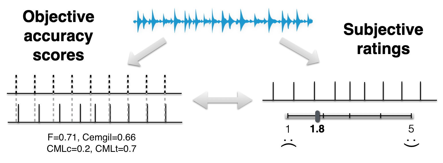
Fig. 4 Overview of objective methods vs subjective ratings
F-measure
Among the most used evaluation methods is the F-measure, which is also widely adopted in onset detection, structural boundary detection and other temporal MIR tasks. A high-level graphical overview is shown below.
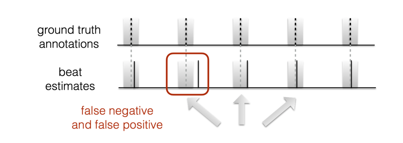
Fig. 5 F-measure
For beat tracking, we typically use a tolerance window of +/- 70ms around each ground truth annotation.
Beats that uniquely fall into these tolerance windows are true positives (or hits).
Any additional beats in each tolerance window, or those outside of any tolerance window, counted as false positives.
Finally, any empty tolerance windows with no beats are counted as false negatives.
With these three quantities we can calculate the precision and recall and in turn the F-measure.
However, if we choose the vary the size of the tolerance window we can dramatically change these quantities. Make it too wide, and we’ll treat very poorly localised beats as accurate, and by contrast too narrow, and we’ll mark perceptually accurate beats as errors.
Fig. 6 Animation of F-measure tolerance window
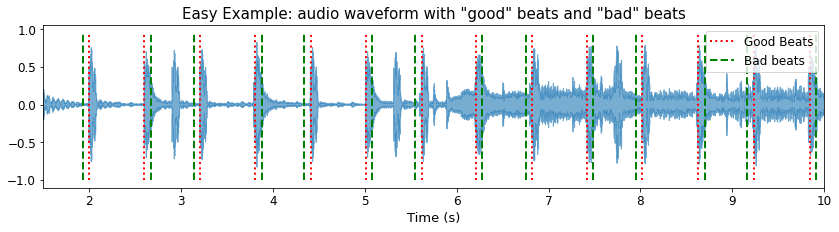
The implication of using a fixed tolerance window is that whenever the beats are uniquely inside and regardless of their temopral location to the annotation, they’re considered accurate. We can push this to a somewhat absurd extreme, by anticipating the even beat annotations by just under 70ms and offseting the odd beat annotations by the same amount.
import warnings
warnings.simplefilter('ignore')
import numpy as np
import librosa
import librosa.display
import IPython.display as ipd
import mir_eval
import matplotlib.pyplot as plt
import scipy.stats


filename = '../assets/ch2_basics/audio/easy_example'

sr = 44100
FIGSIZE = (14,3)

# read audio and annotations
y, sr = librosa.load(filename+'.flac', sr = sr)
ref_beats = np.loadtxt(filename+'.beats')
ref_beats = ref_beats[:,0]
bad_beats = ref_beats.copy()
bad_beats[::2] = bad_beats[::2]-0.069
bad_beats[1::2] = bad_beats[1::2]+0.069

y_good_beats = librosa.clicks(times=ref_beats, sr=sr, click_freq=1000.0,
                              click_duration=0.1, length=len(y))

y_bad_beats = librosa.clicks(times=bad_beats, sr=sr, click_freq=1000.0,
                              click_duration=0.1, length=len(y))

plt.figure(figsize=FIGSIZE)
librosa.display.waveshow(y, sr=sr, alpha=0.6)
plt.vlines(ref_beats, 1.1*y.min(), 1.1*y.max(), label='Good Beats', color='r', linestyle=':', linewidth=2)
plt.vlines(bad_beats, 1.1*y.min(), 1.1*y.max(), label='Bad beats', color='green', linestyle='--', linewidth=2)

plt.legend(fontsize=12);
plt.title('Easy Example: audio waveform with "good" beats and "bad" beats', fontsize=15)
plt.yticks(fontsize=12)
plt.xticks(fontsize=12)
plt.xlabel('Time (s)', fontsize=13)
plt.legend(fontsize=12);
plt.xlim(1.5, 10);
Let’s listen first the unmodified beat annotations.
ipd.Audio(0.6*y[1*sr:10*sr]+0.25*y_good_beats[1*sr:10*sr], rate=sr)
and then the limit of accurate F-measure
ipd.Audio(0.6*y[1*sr:10*sr]+0.25*y_bad_beats[1*sr:10*sr], rate=sr)
We can confirm the F-measure score using mir_eval
print('Fmeasure:', round(mir_eval.beat.f_measure(ref_beats, bad_beats), 3))
Fmeasure: 1.0
Of course, this is a deliberately bad output practically at the limit of what the F-measure calculation will allow, and it’s probably better not to dwell too much on cases like this, but rather accept that this seemingly big tolerance window is useful to catch either: i) natural human variation in tapping and not punish it, or ii) contend with cases like arpeggiated chords (e.g., the first annotated beat in our expressive example) where it’s difficult to mark a single beat location.
Cemgil
An alternative to using a “top-hat” tolerance window is instead to use a Gaussian distribution placed around each annotation. Here we no longer have the notion of a true or false positive, but rather each beat can be assigned the value corresponding to the value of the Gaussian located at the nearest annotation.
In this way, poor localisation like in the “bad beats” example
would be punished since the value of the Gaussian (with standard deviation 40ms as in
the original paper and mir_eval and madmom implementations)
at an offset of +/-70ms will be rather low.
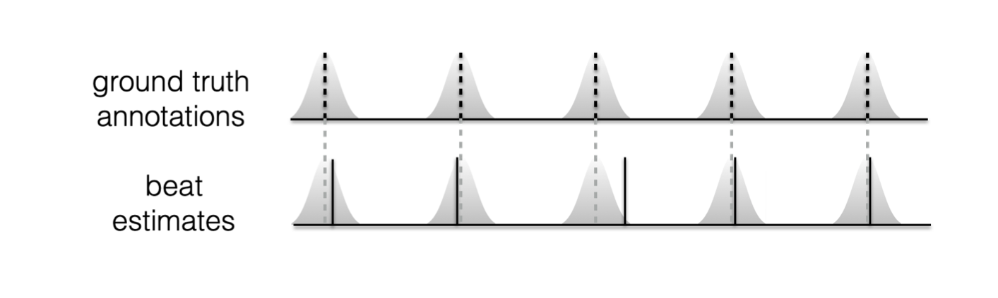
Fig. 7 Cemgil evaluation approach
We can verify this with mir_eval
print('Cemgil:', round(mir_eval.beat.cemgil(ref_beats, bad_beats)[0], 3))
Cemgil: 0.226
And thus we have an F-measure of 1.00 but a Cemgil accuracy of 0.226.
So, how can we use that information to our advantage?
Via the combination of these two scores we can begin to make some interpretation about the qualitative nature of the relationship between estimated beats and annotations. Which in this case would tell us that the metrical level and phase of the beat estimates are the same as the ground truth annotations, but they are poorly localised.
Note
Thus far, we’ve looked at two different, but related, approaches to the evaluation of temporal sequences. We’ve seen too that the F-measure score can be kind of “gamed.” There’s a couple of worthwhile additional perspectives to consider.
Both of these approaches make what we could understand as time-indendent measurements of beat tracking accuracy. Which is to say that each estimated beat is treated as an isolated point in time. So, we have no notion of a beat interval to work with in evaluation. This is largely fine for onset detection and structural boundary detection, but somewhat sub-optimal for temporal data with some strong periodic organisation like musical beats.
What does it mean to score and F-measure or Cemgil accuracy of 0.00? It almost certainly does not mean that there is a totally random relationship between the estimated beats and ground truth annotation, but much more likely that the estimated beats are tapped on the “off-beat” to the annotations.
Continuity-based
With the two points in the above note in mind, we can explore the properties of the “Continuty-based” evaluation approach. Here we make two principal changes:
The first is that we only consider beat i to be accurate if it falls within the tolerance window (more on how that’s defined in a moment) and that beat i-1 also falls within its respective tolerance window, as shown in figure below. Note, in addition we require that the inter-beat-interval also be consistent with the inter-annotation-intereval.
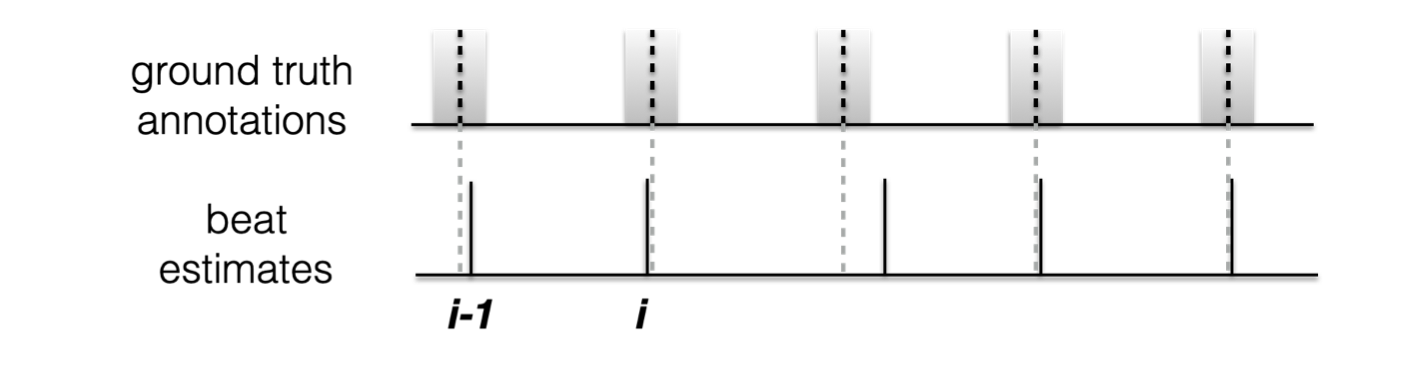
Fig. 8 Overview of contuity based approach
Secondly, and to try to account for some metrical ambiguity in what might be an acceptable sequence of beat estimates, we can generate multiple metrical variations of the annotations and evaluate against each of these in turn, picking the best score available. These metrical variations typically constitute
The same metrical level and “in-phase”
The same metrical level, but tapped on the “off-beat”
Twice the annotated metrical level
Half the annotated metrical level (taking every other annotated beat and starting on the first)
Half the annotated metrical level (taking every other annotated beat and starting on the second)
Depending on the implementation, there may be scope
to allow for a triple and 1/3rd variation as well,
e.g., the evaluation routines in madmom allow for this possibility.
Note
This set of allowed metrical levels bears some similarity to increasing the size of the tolerance window for the F-measure. The more different metrical variations we allow the greater the chance that our beat tracker will hit one of these, even though some might be rather unlikely for a given piece of music.
In the figure below, we demonstrate what happens if the beat estimates are tapped at twice the tempo of the annotations. If we look for continuity between the estimated beat and annotations, we won’t get it, nor at any of the other possibilities except “double” variation.
This means, if we force consistency over the choice of metrical level we’d score precisely 0, but if we take the maximum over these five variations, we could obtain an accuracy of 1.
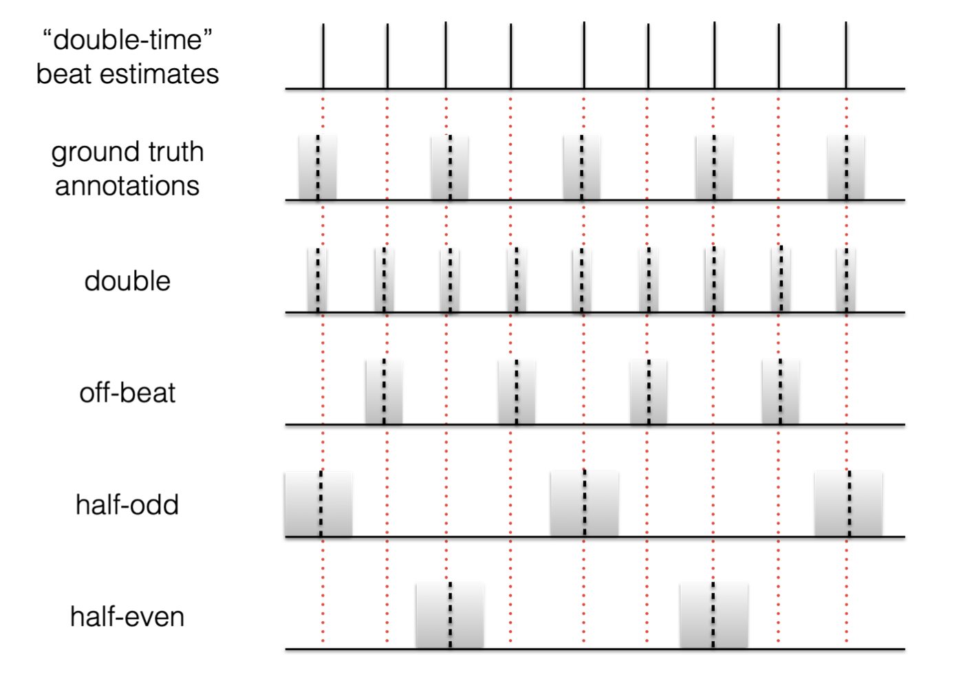
Fig. 9 Example alternative metrical levels for continuity-based evaluation
But what’s going on with those tolerance windows?
Those with keen observation skills will have noticed that the choice of metrical variation has an impact on the width of the tolerance window. As we move to faster metrical levels, the tolerance window shrinks, and as we move to slower metrical levels it gets wider.
This is because the tolerance windows for the continuity-based approach, rather than being calculated in absolute time as in the F-measure (or indeed the parameterisation of the Gaussian for Cemgil’s approach) they are calculated in a beat-relative manner, and set to 17.5% of each inter-annotation-interval.
Finally (yes, we’re still talking about evaluation!) even with all of these factors, we still have two ways in which we can extract an accuracy score.
First, whether we want to take the ratio of the longest continuously correct segment to the length of the excerpt (the “c” variation of CMLc, AMLc)
Or, if we want to take the ratio of the total of the continuously correct segments to the length of the excerpt (the “t” variation of CMLt, AMLt).
So, after all that, we have:
CMLc: “correct” (i.e., annotated) metrical level, with longest single continous segment.
CMLt: “correct” (i.e., annotated) metrical level, with the total of continous segments.
AMLc: “allowed” metrical levels, with longest single continous segment.
AMLt: “allowed” metrical levels, with the total of continous segments.
Based on these scores, we can determine the following:
CMLc <= CMLt and likewise AMLc <= AMLt
CMLc <= AMLc and likewise CMLt <= AMLt
and by virtue of these
CMLc <= AMLt
but
CMLt is not guaranteed to be less than AMLc!
For completeness, let’s return to our “bad beats” and check the scores under the continuity approaches:
print({m:v for m,v in zip(['CMLc', 'CMLt', 'AMLc', 'AMLt'],
                                            mir_eval.beat.continuity(ref_beats, bad_beats))})
{'CMLc': 0.0, 'CMLt': 0.0, 'AMLc': 0.0, 'AMLt': 0.0}
So, 0.0 all round! Since the AMLx scores are zero, we know the CMLx ones must be too. But, we only shifted the bad beats around by just under 70ms, and technically this would be okay according to the +/- 17.5% tolerance windows for phase accuracy. Where this fails is in the periodicity criteria, which is that the inter-beat-intervals alternate between being greater than and less than the allowed inter-annotation-interval.
Beat Evaluation Perspectives
So, after our quick overview of some (but not all) of the available evaluation methods, the question is which should you use? … It depends!
If we know that our algorithm scores highly on CMLc, then we know quite a lot about what that means.
Our algorithm has picked the same metrical level as the one that has been annotated, so we circumvent the chance that the metrical level our beat tracker has picked is “allowed” under the rules, but not appropriate for the individual piece.
We also know that our beat estimates were pretty consistently well-aligned with ground truth annotations.
In situations where CMLt >> CMLc, this can tell us that we’ve got an odd mis-placed beat somewhere and thus we were right most of the time but lapsed just for a moment.
It’s important to stress that this might not be an “error” at all, but an isolated bad annotation in need of correction.
But, ultimately, if we have high confidence in our annotations, then we can do a lot worse than trying to maximise CMLc.
While it’s possible to report a single or set of accuracy scores to summarise the performance of an algorithm, e.g., algorithm X has a mean accuracy of 1000 files = 0.87. We can learn more about its behaviour by:
Plotting its performance over a range of thresholds (i.e., tolerance window sizes)
Looking at visualisations of the relationship between the annotations and the estimated beats so we can pinpoint and understand errors.
On this final point, it may be of interest to look at a very recent approach to evaluation ([PBockCD21] and its open-source implementation here) which determines and visualises the set of steps necessary to transform a beat sequence in such a way that it would maximise the F-measure. In some sense, it tries to replicate and measure the kind of annotation corrections we’ve seen previously in the annotation section.
Extending to tempo and downbeats
The vast majority of this section has looked at issues related to beat tracking evaluation. Indeed, the extension to downbeat estimation is quite straightforward, and frequently the F-measure and Continuity-based evaluation methods are used.
For tempo estimation, it has been commonplace to report two scores: “Acc1” and “Acc2” which verify if an estimated tempo is within +/- 4% of the annotated tempo for Acc1 and likewise for Acc2, but allowing for “octave errors” in the similar way to the “allowed” metrical levels of AMLc/AMLt. However, the recent work of Schreiber et al [SUM20] and the tempo_eval resource have suceeded in moving forward the topic of global tempo evaluation.