On different DNN architectures
Many different architectures have been explored, ranging from MLPs [DBDR15], CNNs [DBDR16, DBDR17, DE16, HG16], RNNs [BockKW14a, KHCW15, ZNY19], Bi-LSTMs [BockKW16], Bi-GRUs [KBockDW16], CRNNs [FMC+19, FMC+18, VDWK17] and recently TCNs [BockD20, BockDK19, MBock19]. But, what have we learned from all this different approaches? Which one works better? What should we take into account when using a particular architecture? Some context and thoughts on this below.
A bit of context
DNNs were introduced in MIR applications motivated by their huge success in computer vision, and due to recent advances that allow for faster training and scalability [GBC16]. The inclusion of these models in MIR tasks has meant a considerable improvement in the performance of automatic systems, in particular tempo, beat and downbeat tracking ones, as can be seen from the MIREX campaigns [JLL19]. Moreover, the use of deep learning models presents other advantages over traditional machine learning methods used in MIR, i.e. they are flexible and adaptable across tasks. As an example, convolutional neural network based models from Computer Vision were adapted for onset detection [SchluterBock14], and then for segment boundary detection [USchluterG14]. Furthermore, DNNs reduce —or allow to remove completely— the stage of hand-crafted feature design, by including the feature learning as part of the learning process.
Note
The adoption of DNNs exacerbated some issues related to the use of supervised learning models: their dependence on annotated data, the bias of the data itself and their lack of interpretability. Annotated data is an important bottleneck in MIR! Especially due to copyright issues, and because annotating a musical piece requires expert knowledge and is thus expensive. Also, models will be biased depending on the dataset used, a problem that also occurs in other learning-based approaches. Besides, deep-learning based methods are usually less interpretable than signal processing methods, making it a bit hard to predict the type of mistakes a DNN would do when presented with e.g. unseen music tracks or genres.
What is a deep net?
In general terms, a deep neural network consists of a composition of non-linear functions that acts as a function approximator \(F_\omega: \mathbf{X} \rightarrow \mathbf{Y}\), for given input and output data \(\mathbf{X}\) and \(\mathbf{Y}\). The network is parametrized by its weights \(\omega\), whose values are optimized so the estimated output \(\hat{\mathbf{Y}}=F_\omega (\mathbf{X})\) approximates the desired output \(\mathbf{Y}\) given an input \(\mathbf{X}\).
Multi-layer perceptrons
Multi-layer perceptrons (MLPs) are the simple and basic modules of DNNs. They are also known as fully-connected layers or dense layers, and consist of a sequence of layers, each defined by an affine transformation composed with a non-linearity:
where \(\mathbf{x} \in \mathbb{R}^{d_{in}}\) is the input, \(\mathbf{y} \in \mathbb{R}^{d_{out}}\) is the output, \(\mathbf{b} \in \mathbb{R}^{d_{out}}\) is called the bias vector and \(\mathbf{W} \in \mathbb{R}^{d_{in} \times d_{out}}\) is the weight matrix. \(f()\) is a non-linear activation function, which allows the model to learn non-linear representations. Note that for multi-dimensional inputs, e.g. \(\mathbf{X} \in \mathbb{R}^{d_1 \times d_2}\), the input is flattened so \(\mathbf{x} \in \mathbb{R}^{d}\) with \(d = d_1 \times d_2\). These layers are usually used to map the input to another space where hopefully the problem (e.g. classification or regression) can be solved more easily.
Note
However, by definition, this type of layer is not shift or scale invariant, meaning that when using this type of network for audio tasks, any small temporal or frequency shift needs dedicated parameters to be modelled, becoming very expensive and inconvenient when it comes to modelling music.
MLPs have been mainly used in early works before convolutional neural networks (CNNs) and recurrent neural networks (RNNs) became popular [CFCS17], and are now used in combination with those architectures, usually as the last layers of a model to map high dimensional intermediate representations to the output space (e.g. classes), as discussed below.
Convolutional Neural networks
The main idea behind CNNs is to convolve their input with learnable kernels. Systems based on CNNs make the most of the capacity of such networks to learn invariant properties of the data while needing fewer parameters than other DNNs such as MLPs and being easier to train. Also, convolutions are suitable for retrieving changes in the input representations, which are (usually) indicators of beat and/or downbeat positions (e.g. changes in harmonic content or spectral energy). Besides, CNNs have shown to be good high-level feature extractors in music [DBDR17], and are able to express complex relations.
CNNs can be designed to perform either 1-d or 2-d convolutions, or a combination of both. In the context of audio, in general 1-d convolutions are used in the temporal domain, whereas 2-d convolutions are usually applied to exploit time-frequency related information. We will focus on models that perform 2-d convolutions. The output of a convolutional layer is usually called feature map. In the context of audio applications, it is common to use CNN architectures combining convolutional and pooling layers. Pooling layers are used to down-sample feature maps between convolutional layers, so that deeper layers integrate larger extents of data. The most widely used pooling operator in the context of audio is max-pooling, which samples —usually— non-overlapping patches by keeping the biggest value in that region.
Note
The main disadvantage of CNNs is their lack of long-term context, which restrict the musical context and interplay with temporal scales that could improve their performance. This can be improved by combining CNNs with RNNs [FMR+19, FMC+18, VDWK17].
A convolutional layer is given by the following expression:
where all \(\mathbf{Y}^j\), \(\mathbf{W}^{jk}\), and \(\mathbf{X}^k\) are 2-d, \(\mathbf{b}\) is the bias vector, \(j\) indicates the j-th output channel, and \(k\) indicates the k-th input channel. The input is a tensor \(\mathbf{X} \in \mathbb{R}^{T\times F \times d}\), where \(T\) and \(F\) refer to the temporal and spatial—usually frequency—axes, and \(d\) denotes a non-convolutional dimension or channel. In most audio applications \(d\) usually equals one, though sometimes is used to encode multiple channels or multiple representations of the input (e.g. each channel is one representation). Note that while \(\mathbf{Y}\) and \(\mathbf{X}\) are 3-d arrays (with axes for height, width and channel), \(\mathbf{W}\) is a 4-d array, so \(\mathbf{W} \in \mathbb{R}^{h \times l \times d_{in} \times d_{out}}\), \(h\) and \(l\) being the dimensions of the convolution, and the 3rd and 4th dimensions account for the relation between input and output channels.
Tip
CNNs are suitable to problems that have two characteristics [McF18]: statistically meaningful information tends to concentrate locally (e.g. within a window around an event), and shift-invariance (e.g. in time or frequency) can be used to reduce model complexity by reusing kernels’ weights with multiple inputs.
Recurrent networks
Many approaches exploited recurrent neural networks given their suitability to process sequential data. In theory, recurrent architectures are flexible in terms of the temporal context they can model, which makes them appealing for music applications. In practice there are some limitations on the amount of context they can effectively learn [GTH19], and although it is clear that they can learn close metrical levels such as beats and downbeats [BockKW16], is not clear if they can successfully learn interrelationships between farther temporal scales in music.
Unlike CNNs which are effective at modelling fixed-length local interactions, recurrent neural networks (RNNs) are good in modelling variable-length long-term interactions. RNNs exploit recurrent connections since they are formulated as [GBC16]:
where \(\mathbf{h}_t\) is a hidden state vector that stores information at time \(t\), \(f_y\) and \(f_h\) are the non-linearities of the output and hidden state respectively, and \(\mathbf{W}_y, \mathbf{W}_h\) and \(\mathbf{U}\) are matrices of trainable weights. An RNN integrates information over time up to time step \(t\) to estimate the state vector \(\mathbf{h}_t\), being suitable to model sequential data. Note that learning the weights \(\mathbf{W}_y, \mathbf{W}_h\) and \(\mathbf{U}\) in a RNN is challenging given the dependency of the gradient on the entire state sequence [McF18]. In practice, back-propagation through time is used [W+90], which consists in unrolling the equation above up to \(k\) time steps and applying standard back propagation. Given the accumulative effect of applying \(\mathbf{U}\) when unrolling the equation above, the gradient values tend to either vanish or explode if \(k\) is too big, a problem known as the vanishing and exploding gradient problem. For that reason, in practice the value of \(k\) is limited to account for relatively short sequences.
Note
The most commonly used variations of RNNs, that were designed to mitigate the vanishing/exploding problem of the gradient, include the addition of gates that control the flow of information through the network. The most popular ones in MIR applications are long-short memory units (LSTMs) [HS97] and gated recurrent units (GRUs) [CVMerrienboerG+14]. Since they show similar empirical results, we only discuss GRUs below.
Gated recurrent units
In a GRU layer, the gate variables \(\mathbf{r}_t\) and \(\mathbf{u}_t\) —named as reset and update vectors— control the updates to the state vector \(\mathbf{h}_t\), which is a combination of the previous state \(\mathbf{h}_{t-1}\) and a proposed next state \(\hat{\mathbf{h}}_t\). The equations that rule these updates are given by:
\(\odot\) indicates the element-wise Hadamard product, \(f_g\) is the activation applied to the reset and update vectors, and \(f_h\) is the output activation. \(\mathbf{W}_r, \mathbf{W}_u, \mathbf{W}_h \in \mathbb{R}^{d_{i-1}\times d_i}\) are the input weights, \(\mathbf{U}_r, \mathbf{U}_u, \mathbf{U}_h \in \mathbb{R}^{d_{i}\times d_i}\) are the recurrent weights and \(\mathbf{b}_r, \mathbf{b}_u, \mathbf{b}_h \in \mathbb{R}^{d_{i}}\) are the biases. The activation functions \(f_g\) and \(f_h\) are typically sigmoid and tanh, since saturating functions help to avoid exploding gradients in recurrent networks.
The GRU operates as follows: when \(\mathbf{u}_t\) is close to 1, the previous observation \(\mathbf{h}_{t-1}\) dominates in the equations above. When \(\mathbf{u}_t\) gets close to 0, depending on the value of \(\mathbf{r}_t\), either a new state is updated with the standard recurrent equation by \(\hat{\mathbf{h}}_t = f(\mathbf{W}_h \mathbf{x}_t + \mathbf{v}_h \mathbf{h}_{t-1} + \mathbf{b}_h)\), if \(\mathbf{r}_t=1\), or the state is reset as if the \(\mathbf{x}_t\) was the first observation in the sequence by \(\hat{\mathbf{h}}_t = f(\mathbf{W}_h \mathbf{x}_t + \mathbf{b}_h)\).
Tip
The reset variables allow GRUs to successfully model long-term interactions, and perform comparably to LSTMs, but GRUs are simpler since LSTMs have three gate vectors and one extra memory gate. Empirical studies show that both networks perform comparably while GRUs are faster to train [GSKoutnik+16, JZS15].
Bi-directional models
GRUs and RNNs in general are designed to integrate information in one direction, e.g. in an audio application they integrate information forward in time. However, it can be beneficial to integrate information in both directions, and so has been the case for neural networks in audio applications such as beat tracking [BockS11] or environmental sound detection [PHV16]. A bi-directional recurrent neural network (Bi-RNN) [SP97] in the context of audio consists of two RNNs running in opposite time directions with their hidden vectors \(\mathbf{h}_t ^f\) and \(\mathbf{h}_t ^b\) being concatenated, so the output \(h_t\) at time \(t\) has information about the entire sequence. Unless the application is online, Bi-RNNs are usually preferred due to better performance [McF18].
Temporal Convolutional networks
A “simple” convolution is only able to consider the context up to a size linear in the depth of the network. This makes it challenging to apply them on sequential data, because the amount of context they can handle is small. In the context of beat and downbeat tracking systems, that might mean that the input granularity should be coarser if we want to guarantee that enough context is taken into account for e.g. downbeat tracking. Instead, Temporal Convolutional Networks (TCNs) [BKK18] use dilated convolutions which enable exponentially large receptive fields! Formally, for a 1-D sequence input \(\mathbf{x} \in \mathbb{R}^d_{in}\) and a filter \(f : \{0, \dots, k − 1\} \rightarrow \mathbb{R}\), the dilated convolution operation \(F\) on element \(s\) of the sequence is defined as:
where \(d\) is the dilation factor, \(k\) is the filter size, and \(s − d ·i\) accounts for the direction of the past. Dilation is equivalent to introducing a fixed step between every two adjacent filter taps, i.e. skipping samples in the audio. When \(d = 1\), a dilated convolution becomes a regular convolution.
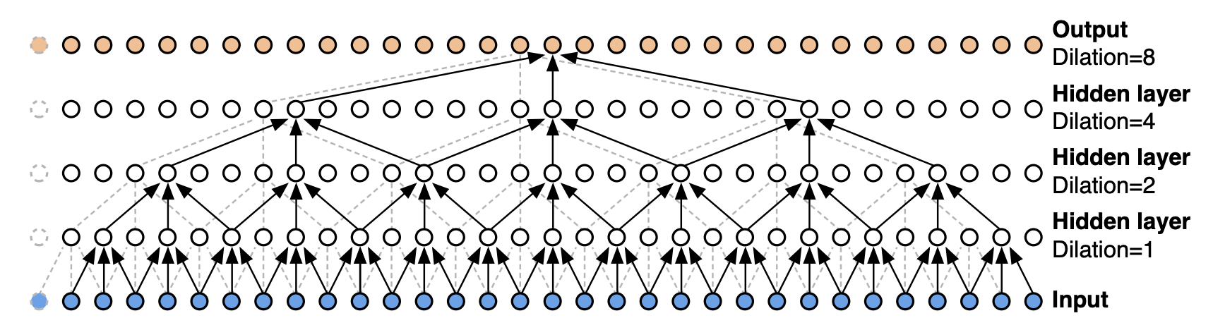
Intuitively, TCNs perform convolutions across sub-sampled input representations and are good at learning sequential/temporal structure, since they retain the parallelisation property of standard CNNs but can handle much more context. Besides, TCNs can be trained far more efficiently than a RNN, LSTM or GRU from a computational perspective, and with much less number of weights. Given this advantages, TCNs are taking over these recurrent networks in many sequential tasks.
SPOILER ALERT!!
Because of being light, fast to train and have great performance, we’re using TCNs for the hands on part of the tutorial!
Hybrid architectures
As mentioned before, MLPs are now usually being used in combination with CNNs, which are able to overcome the lack of shift and scale invariance MLPs suffer. At the same time, MLPs offer a simple alternative for mapping representations from a big-dimensional space to a smaller one, suitable for classification problems.
Finally, hybrid architectures that integrate convolutional and recurrent networks have recently become popular and have proven to be effective in audio applications, especially in MIR [MB17, SBD16]. They integrate local feature learning with global feature integration, a playground between time scales that is in particular interesting for beat and downbeat tracking.
Learning and optimization
To optimize the parameters \(\omega\), a variant of gradient descent is usually exploited. A loss function \(J(\omega)\) measures the difference between the predicted and desired outputs \(\hat{\mathbf{Y}}\) and \(\mathbf{Y}\), so the main idea behind the optimization process is to iteratively update the weights \(\omega\) so the loss function decreases, that is:
Where \(\eta\) is the learning rate which controls how much to update the values of \(\omega\) at each iteration. Because the DNN consists of a composition of functions, the gradient of \(J(\omega)\), \(\nabla \omega J(\omega)\), is obtained via the chain rule, a process known as back propagation. In the last four years, many software packages that implement automatic differentiation tools and various versions of gradient descent were released, [AAB+15, C+15, TheanoDTeam16], reducing considerably the time needed for the implementation of such models.
Since computing the gradient over a large training set is very expensive both in memory and computational complexity, a widely adopted variant of gradient descent is Stochastic Gradient Descent (SGD) [Bot91], which approximates the gradient at each step on a mini-batch of training samples, \(B\), considerably smaller than the training set. There are other variants of SGD such as momentum methods or adaptive update schemes that accelerate convergence dramatically, by re-using information of previous gradients (momentum) and reducing the dependence on \(\eta\). From 2017, the most popular method for optimizing DNNs has been the adaptive method ADAM [KB14].
Another common practice in the optimization of DNNs is to use early stopping as regularization [SjobergL95], which means to stop training if the training –or validation– loss is not improving after a certain amount of iterations. Finally, batch normalization (BN) [IS15] is widely used in practice as well, and consists of scaling the data by estimating its statistics during training, which usually leads to better performance and faster convergence.
Activation functions
The expressive power of DNNs is in great extent due to the use of non-linearities \(f()\) in the model. The type of non-linearity used depends on whether it is an internal layer or the output layer. Many different options have been explored in the literature for intermediate-layer non-linearities —usually named transfer functions, the two main groups being saturating or non-saturating functions (e.g. tanh or sigmoid for saturated, because they saturate in 0 and 1, and rectified linear units (ReLUs) [NH10] for non-saturating ones). Usually non-saturating activations are preferred in practice for being simpler to train and increasing training speed [McF18].